ResistXplorer is a user-friendly, comprehensive web-based tool for analyzing data sets generated from
AMR metagenomics studies. The focus of this tool is to perform visual, statistical and exploratory analysis of
resistome data. It is designed to support five kinds of analysis:
Compositional profiling: provides various analyses commonly used in community ecology such as alpha diversity,
rarefaction curves or ordination analysis, coupled with various intuitive visualization support
(interactive sankey diagram, zoomable sunburst, treemap, stacked bar or area plots) to assist
users gain a comphrehensive view of the composition of their uploaded resistome profiles.
Functional profiling: supports analysis and profiling of resistome at various functional
categories or levels (e.g. Drug class, Mechanism) to help users acheive more biological and
actionable insights together with a better understanding of their data.
Comparative analysis: providing multiple standard as well as more advanced (CoDA-based)
normalization techniques coupled with differential analysis
approaches (edgeR, DEseq2, LEfSE, metagenomeSeq, ANCOM and ALDEx2) to
detect features (ARGs) that are significantly different between conditions under investigation.
Integrative analysis: enable users to integrate thier paired resistome and microbiome
abundance profiles for understanding the complex interplay as well as exploring the potential
associations between microbial ecology and AMR using several univariate and multivariate
omics integration statistical methods.
ARGs-microbial host network exploration: allow users to intuitively explore the
microbial hosts and functional associations of their uploaded list of
antimicrobial resistance genes (ARGs) using a powerful and fully featured
network visual analytics system to obtain better interpretation of AMR
resistance mechanisms and information on possible dissemination routes of
ARGs.
ResistoXplorer supports most common format generated in metagenomic-based AMR studies i.e.,
count abundance tables (ARG/OTU/taxa), together with metadata and annotation files.
Users can found the detailed descriptions, example datasets and screenshots on the Data Format page.
ResistoXplorer is explicitly designed for downstream analysis and currently does not
accept raw sequencing data. The annotated ARG count or abundance table obtained after
preprocessing and upstream analysis of metagenomic sequencing data is the standard input for ResistoXplorer.
For shotgun metagenomics data, there are several bioinformatics pipelines for processing the raw sequence data into an ARG count table. For instance,
AMRPlusPlus: is a Galaxy-based metagenomics pipeline that uses current and new tools to help
identify and quantify ARGs within metagenomic sequence data to generate count table in text format.
ARG-OAPs: it utilizes the SARG database and a hybrid functional gene annotation pipeline to do
fast annotation and classification of ARG-like sequences from metagenomic data.
DeepARG: is a fully automated data analysis pipeline for antibiotic resistance annotation of metagenomic data using the deepARG algorithm and deepARG-DB database.
For more information on available methods and databases for resistome annotation, please refer to the
review articles by Moolchandani, B et al.
and Gupta, CL et al.
The purpose of data filtering is to allow users to remove low quality and/or uninformative features to improve
downstream statistical analysis. ResistoXplorer contains three data filtering procedures:
Minimal data filtering - the procedure will remove features containing all zeros, or appearing in only one sample with very extremely low counts (considered as artifacts).
These extremely rare features should be removed from analysis due to biological and technical considerations. It applies to all analysis except alpha and rarefaction analysis;
Low abundance features - features that are present in a few samples with very low read counts are may be due to sequencing errors or low-level contaminations;
Low variance features - features with constant variance across all the samples are unlikely to be associated with the conditions under study;
Users can choose from low count abundance filter options to filter features with very small counts in very few sample (i.e. low prevalence).
If primary purpose is comparative analysis, users should filter features that exhibit low variance based on
inter-quantile range, standard deviation or coefficient of variation, as they are very unlikely to be significant
in the comparative analysis.
The Data Inspection page provides the text summary and statistics of the uploaded files (Text Summary tab) along with graphically describing the read counts for all uploaded samples (Library Size Overview tab),
which are informative in selecting or choosing the appropriate filtration method and their cutoff based on the data.
Metagenomic data possess some unique characteristics such as vast differences in sequencing depth, sparsity, skewed distributions,
over-dispersion and compositionality. Hence, it is critical
to normalize the data to achieve comparable and meaningful results. To deal with these issues, ResistoXplorer supports three kind of
normalization approaches such as:
Rarefaction: this method deals with uneven sequencing depths by randomly removing reads in the different samples until the sequencing depth is equal in all samples.
Scaling-based methods: these methods account for uneven sequencing depths by deriving a sample-specific scaling factor for bringing samples to the same scale for comparison.
Transformation-based: it includes approaches to deal with sparsity, compositionality, and large variations within the count data.
ResistoXplorer supports a variety of methods for data normalization. A brief summary is provided below:
Rarefaction: this method deals with uneven sequencing depths by randomly removing
reads in the different samples until the library size of all the samples are same as sample with
lowest sequencing depth. Whenever the library size of the samples varies too much (i.e., >10X),
it is recommended to perform rarefaction before normalizing your data. It also seems to perform better during ordination or clustering analysis.
For more details, please refer to paper by Weiss, S et al.
Total Sum Scaling (TSS) normalization: this method removes technical bias related to different
sequencing depth in different libraries via simply dividing each feature count with the
total library size to yield relative proportion of counts for that feature.
For easier interpretation, we can multiply it by 1,000,000 to get the number of reads
corresponding to that feature per million reads. It is also known as Count per Million (CPM) normalization. LEfSe utilizes
this kind of approach for normalizing data before conducting statistical testing.
Log Count per million (CPM) normalization: this method perform log transformation on count per million normalized data
in order to deal with large variance in count distributions in addition to library size differences.
his kind of approach is been used by R packages such as edgeR and voom which are designed for
identifying differentially abundant genes in RNA-Seq count data.
Cumulative Sum Scaling (CSS) normalization: this method corrects for differences in library size by calculating the scaling factors
as the cumulative sum of gene abundances up to a data-derived threshold to remove the variability in data caused by highly abundant genes.
By default, metagenomeSeq utilizes this approach for differential analysis.
Relative proportion: this approach computes the relative proportion of a feature by dividing each feature count
by the total number of counts (library size) per sample.
Relative log expression (RLE) normalization: this method estimates the median library from the geometric mean of the
gene-specific abundances over all samples. The median ratio of each sample to the median library is used as the
scaling factor. By default, DESeq2 utilizes this approach for identifying differentially abundant genes. This method was proposed by Anders & Huber.
Trimmed mean of M-values (TMM) normalization: this method is proposed by Robinson & Oshlack, where the scaling factor is derived using
a weighted trimmed mean over the differences of the log-transformed gene-count fold-change
(relative abundance) between the samples. By default, edgeR utilizes this approach for differential analysis in ResistoXplorer.
Upper Quantile normalization: this approach calculates the scaling factors from the 75th percentile of the gene count distribution for each
library, after removing genes which are zero in all libraries. This method is derived from edgeR package
proposed by this method proposed by Bullard et al.
Hellinger Transformation: this method computes the relative proportion of a feature by dividing each feature count by the total number of counts
(library size) per sample, and then taking the square root of it.
Log-Ratio (CLR and ALR) Transformation: these methods are specifically designed to normalize compositional data. They transforms the relative
abundances of each element, or the values in the table of counts for each element, to ratios between all parts by using either geometric mean of
the sample or single element as the reference. Further, taking the logarithm of these ratios, brings the data in a Euclidean (real) space,
such that standard statistical methods can be applied. CoDA-based methods such as ALDEx2 and ANCOM utilize this approach for normalizing data before conducting statistical testing.
There is no consensus guideline with regard to which normalization performs the best and should be used for all types of datasets.The choice of method is dependent upon the type of analyses to be performed. Users can explore different
approaches and visually investigate the clustering patterns (i.e., ordination plots, dendrogram and heatmap) to determine the effects of different normalization methods with regard to the experimental factor of interest.
For detailed discussion about these methods and their performance on different type of analyses, users are referred to these comparative studies by
Pereira, MB et al., Jonsson, V et al., Weiss, S et al. and McMurdie, PJ et al.
The normalized data is used for exploratory data analysis including ordination, clustering and integrative analysis .
Also, differential abundance testing using different approaches are performed on normalized data. However, each of these methods
will use their own specific normalization procedure. For example, the relative log expression (RLE) normalization is used for DESeq2,
and the centered log-ratio transformation is applied for ALDEx2.
Whenever the library size or sequencing depth of your samples differ from each other by more than 10 fold, it is recommended to perform
rarefaction before normalizing your data. Such issue cannot be addressed by normalization methods directly. Note, users should also consider to
remove the shallow sequenced samples as such gross difference could be due to experimental failure. For more details, please
refer to the paper by Weiss, S et al. In ResistoXplorer,
users can directly visualize the Library size (available on the Data Inspection page) or either perform rarefaction curve
analysis to determine the sequencing depth with respect to number of ARGs (features) detected for each sample in order to check the need of rarefaction for their data.
Unassigned category contain features without or missing (have NA) annotation at certain functional level. For instance, if you are looking at
Class level, and 20% of the features do not have a Class-level annotation, these are merged together as Unassigned.
Outliers refers to those samples that are significantly different from the "majority".
The potential outlier will distinguish itself as the sample located far away from major
clusters or trends formed by the remaining data. To discover potential outliers, users can
use a variety of summary plots to visualize their data. For instance, a sample with extreme
diversity (alpha or ordination) or very low sequencing depth (rarefaction curve analysis or Library size overview)
may be considered a potential outlier. Outliers may be arise due to either biological or technical reasons. To deal with outliers,
the first step is to check if those samples were measured properly. In many cases, outliers are
the result of operational errors during the analytical process. If those values cannot be corrected
(i.e. by normalization procedures), they should be removed from your analysis.
Alpha diversity is an ecology-based analysis used to measure the diversity within a sample. It summarizes both the feature richness (total number of features) and/or evenness
(abundance distribution across features) within a sample. Eight alpha diversity measures are currently supported
in ResistoXplorer, each assessing different aspects of the community. For instance, Observed calculates the total number of
unique features found in each sample, whereas Chao1 and ACE estimate feature richness by accounting for features that are unobserved
because of low abundance. Shannon and Simpson measure take both feature richness and evenness into account, with varying
weight given to evenness. Further details on different diversity measures can be found here.
The recent comparative study by Palme, JB et al. suggested that Chao1 estimator performed very well and recommended to use for estimating
ARG diversity, while the performance of other measures such as Shannon, Simpson and ACE indices was not very satisfactory.
These bars basically represent the Standard Error (SE) in calculating the alpha diversity.
Metrices that estimate a SE include ACE and Chao1, which are used as similarity estimators, allowing
for rigorous comparison of two or more similarity index values. SEs are computed by a bootstrap procedure,
which requires resampling the observed data and recomputing the estimators many times.
Currently, users can calculate dissimilarities between samples using five (including euclidean) commonly used non-phylogenetic-based quantitative or
qualitative distance measures. The Jaccard distance utilizes just the presence or absence of features to estimate
differences in resistome composition; Bray-Curtis dissimilarity uses abundance data and calculates
differences in feature abundance; Jensen-Shannon divergence calculates the distance between two probability
distributions that account for the presence and abundance of resistome features. Further details on different measures can be found
here.
Since the different types of distance measures have specific niches and can
affect the outcomes and the interpretation of the analysis, it is recommended to apply
different measures to better understand the factors underlying composition differences. For more details, please refer to
papers by Goodrich, K et al. and
Kuczynski, J et al.
Currently, three widely accepted ordination methods are supported for visualization of distance matrix at low-dimensional space (i.e., 2D-3D plots), including principal coordinate analysis (PCoA),
non-metric multidimensional scaling (NMDS) and principal component analysis (PCA). Both PCoA and NMDS take the distance matrix as an input.
PCoA maximizes the linear correlation between samples, while NMDS maximizes the rank-order correlation between
samples. Users should use PCoA if distances between samples are so close that a linear transformation
would be enough. NMDS is recommended if users wanted to highlight the gradient structure within their data. While, PCA is
just a type of PCoA that uses euclidean distance. In particular, users can follow a
CoDA ordination approach by performing PCA on the centered log-ratio transformed data.
ResistoXplorer supports both standard as well as more recent compositional data analysis (CoDA) based univariate analysis
approaches such as: edgeR, DESeq2, metagenomeSeq, LEfSe, ALDEx2 and ANCOM.
EdgeR and DESeq2 are both well-established and robust methods developed for RNA-Seq data, that also perform well for metagenomic data.
The differences between them rely mostly on their normalization method and the algorithms used for estimation of dispersion.
While edgeR moderates the dispersion estimate for each gene toward a common estimate across all genes using a weighted
conditional likelihood, DESeq2 detects and corrects dispersion estimates that are too low through modeling of the
dependence of the dispersion on the average expression strength over all samples. In general, DESeq2 is more
robust in estimating differential expression features and usually yields a low false positive rate, while
edgeR is more powerful, but it can also lead to higher rates of false detection. For more details about their implementation please refer to
DESeq2 and
EdgeR
papers.
metagenomeSeq is primarily designed to estimate differential abundance in sparse high-throughput microbial marker-gene survey data. This approach uses a
combination of Cumulative Sum Scaling (CSS) normalization with zero-inflated Gaussian distribution mixture or zero-inflated Log-Normal mixture model
to account for undersampling in large-scale metagenomic studies. For more details, please refer to the original paper here:
metagenomeSeq.
There are two statistical models implemented in metagenomeSeq to model the data:
fitFeature: It is based on a zero-inflated Log-Normal mixture model. This approach is recommended by the author.
This model currently only supports two-group comparisons.
fitZig: It is based on a zero-inflated Gaussian mixture model. It can be used when multiple groups are present
for differential abundance testing.
LDA Effective Size (LEfSe) is a biomarker discovery and explanation method for high-dimensional data. It couples standard tests for statistical significance along with
other methods for biological consistency and effect size estimation. Firstly, it uses the non-parametric factorial
Kruskal-Wallis (KW) sum-rank test to detect features with significant differential abundance with respect to
the class of interest; biological consistency is subsequently investigated using a set of pairwise tests among
subclasses using the (unpaired) Wilcoxon rank-sum test. As a last step, LEfSe uses Linear Discriminant Analysis (LDA) to estimate the
effect size of each differentially abundant feature. The result consists of a table listing all the features, the logarithmic value of the highest mean among all the classes,
and if the feature is discriminative, the class with the highest mean and the logarithmic LDA score (Effect Size).
For more details, please refer to the original paper here: LEfSe
ANCOM (analysis of composition of microbiomes) is used for detecting differences in microbial
mean taxa abundance. In ResistoXplorer, it has been adapted to analyze the
composition of resistomes. The methodology tests the log-ratio abundance (to account for compositionality) of all pairs of
features for differences in means using nonparametric statistical tests. The number of significant
results involving each feature is used to calculate its significance.
For more details, please refer to the original paper here: ANCOM
The W value is basically just a count of number of sub-hypotheses than have been passed for a given feature. For instance,
if you have 500 features, and W=20, for feature x, then sub-hypotheses is passed 20 times. This means, that the ratio feature
x and 20 other features were detected to be significantly different across the conditions under study. For more details, please
refer to the discussion forum here.
ALDEx2 is implemented as R package to work with differential abundance analysis for the comparison of two or
more conditions. It utilizes a Dirichlet-multinomial model that uses counts to infer abundance.
This is optimized for three or more experimental replicates. The method infers biological and
sampling variation to calculate the expected false discovery rate, given the variation,
based on a Wilcoxon Rank Sum test and Welch's t-test (for two groups), and a Kruskal-Wallis test,
a generalized linear model, or a correlation test (for more than two groups).
For more details, please refer to the original paper here: ALDEx2
Choosing the appropriate statistical method for identifying differentially abundant genes in metagenomic data, depends upon the data characteristics (sample or group size, sequencing depth, effect sizes, genes abundances, etc.) of a given study.
Currently, there is no one single statistical method that is suitable for all types of metagenomic datasets.
The following guidelines are based on the comparative studies performed by Weiss, S et al. and Jonsson, V et al. on
microbiome and metagenomic data. Such large scale benchmarking studies are often constructive, and should be read and carefully analyze to make final decision on which method to choose for users own data.
DESeq2 and edgeR has the highest power to compare groups, especially for small group (<20 samples per group) and even library sizes;
MetagenomeSeq’s fitZIG is a faster alternative to DESeq2 for larger group sizes (>50 samples per group);
For larger sample sizes (>50 samples), rarefying coupled with a non-parametric test, such as the Mann-Whitney test, can also yield equally high sensitivity;
ANCOM is more stable in terms of false discovery rates (FDR) for a wide range of sample sizes.
The Random Forest algorithm uses an ensemble of classification trees (forest) where each tree is grown based
on a random subset of features from a bootstrap sample at each branch. The final class prediction is based
on the majority vote of the ensemble. The unbiased estimate of classification errors is obtained by
aggregating cross-validation results using bootstrapped samples while the forest is being constructed.
Random forest also measure the importance of each feature based on the increase of the error when it is
randomly re-shuffled. It can indicate which groups are easier to predict based on errors.
A graphical output is generated to summarize its classification performance. More details about Random Forest can be found
here.
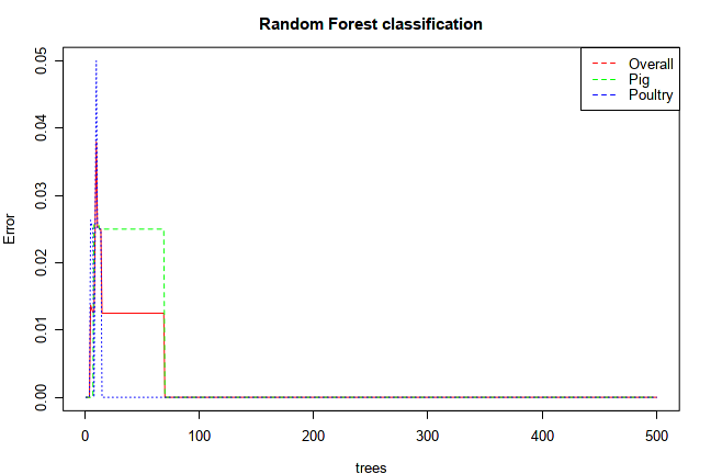
The graphical output from Random Forests shows the changes of error rates with regard to the number of trees as the forests built.
It can indicate when the performance will stabilize after certain number of trees. Users can also see which group tend to have
higher error rates, which group is relatively easy to predict. For instance, the example below shows that using ~70 trees, the
algorithm can achieve perfect prediction for each group.
SVM algorithm seeks to find a nonlinear decision function (hyperplane) by projecting data into higher dimensional feature
space and separating it by means of a maximum margin hyperplane. The SVM analysis is performed using recursive
feature selection and sample classification via linear kernel. Features are selected based on their relative
contribution in the classification using cross-validation error rates. The features which hold less variance
(least significant) are removed in the successive steps. This procedure generates a series of SVM models (levels).
The features used by the best model are considered to be important and ranked based on their frequencies of
being selected in the model (also plotted). More details about SVM can be found
here.
The position of the nodes within the network will reveal their importance in terms of connection with
other antibiotic resistance genes and microbial hosts. Consequently, changes in the most important
positions of the network will have more impact as opposed to less important or more peripheral positions.
This means that if you try to ‘click and drag’ an important node, it will carry several other smaller
nodes with it. Their position will not change, but you will see that the lines connecting them
follow the more important node. The degree centrality indicates the number of connections to
other nodes (the node with the highest degree of centrality will act as a hub of the network),
while the betweenness centrality measures the number of shortest paths going through the node considering
the whole network (the node with the highest betweenness centrality controls the flow of information in the network).
Each of the measures is independent. In addition, you can also double click several nodes to select them, and extract
them to a new network. With this, you can focus on your ARGs of interest. Or you can use this to analyze parts of
the network separately.